Computing Overlap Masks
Defining a region mask within its bounding box
For aperture photometry, a common operation is to compute, for a given image and region, a mask or array of pixel indices defining which pixels (in the whole image or a minimal rectangular bounding box) are inside and outside the region.
All PixelRegion objects have a
to_mask() method that returns a
RegionMask object that contains information about
whether pixels are inside the region, and can be used to mask data
arrays:
>>> from regions.core import PixCoord
>>> from regions.shapes.circle import CirclePixelRegion
>>> center = PixCoord(4., 5.)
>>> reg = CirclePixelRegion(center, 2.3411)
>>> mask = reg.to_mask()
>>> mask.data
array([[0., 1., 1., 1., 0.],
       [1., 1., 1., 1., 1.],
       [1., 1., 1., 1., 1.],
       [1., 1., 1., 1., 1.],
       [0., 1., 1., 1., 0.]])
The mask data contains floating point that are between 0 (no overlap) and 1 (full overlap). By default, this is determined by looking only at the central position in each pixel, and:
>>> reg.to_mask()
is equivalent to:
>>> reg.to_mask(mode='center')
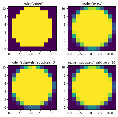
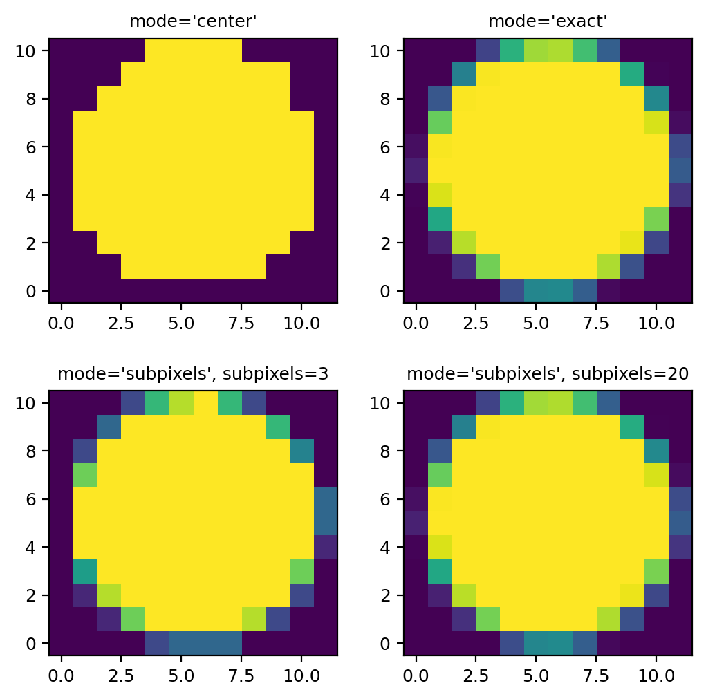
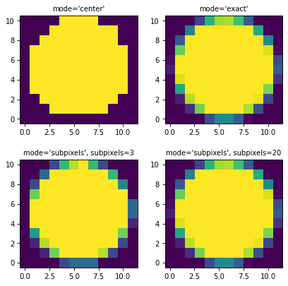
The other mask modes that are available are:
mode='exact': the overlap is determined using the exact geometrical overlap between pixels and the region. This is slower than using the central position, but allows partial overlap to be treated correctly. The mask data values will be between 0 and 1 for partial-pixel overlap.mode='subpixels': the overlap is determined by sub-sampling the pixel using a grid of sub-pixels. The number of sub-pixels to use in this mode should be given using thesubpixelsargument. The mask data values will be between 0 and 1 for partial-pixel overlap.
Here are what the region masks produced by different modes look like:
import matplotlib.pyplot as plt
from regions.core import PixCoord
from regions.shapes.circle import CirclePixelRegion

center = PixCoord(26.6, 27.2)
reg = CirclePixelRegion(center, 5.2)

plt.figure(figsize=(6, 6))

mask1 = reg.to_mask(mode='center')
plt.subplot(2, 2, 1)
plt.title("mode='center'", size=9)
plt.imshow(mask1.data, cmap=plt.cm.viridis,
           interpolation='nearest', origin='lower')

mask2 = reg.to_mask(mode='exact')
plt.subplot(2, 2, 2)
plt.title("mode='exact'", size=9)
plt.imshow(mask2.data, cmap=plt.cm.viridis,
           interpolation='nearest', origin='lower')

mask3 = reg.to_mask(mode='subpixels', subpixels=3)
plt.subplot(2, 2, 3)
plt.title("mode='subpixels', subpixels=3", size=9)
plt.imshow(mask3.data, cmap=plt.cm.viridis,
           interpolation='nearest', origin='lower')

mask4 = reg.to_mask(mode='subpixels', subpixels=20)
plt.subplot(2, 2, 4)
plt.title("mode='subpixels', subpixels=20", size=9)
plt.imshow(mask4.data, cmap=plt.cm.viridis,
           interpolation='nearest', origin='lower')
(Source code, png, hires.png, pdf, svg)
As we’ve seen above, the RegionMask object has a
data attribute that contains a Numpy array with the mask values.
However, if you have, for example, a small circular region with a radius
of 3 pixels at a pixel position of (1000, 1000), it would be inefficient
to store a large mask array that has a size to cover this position (most
of the mask values would be zero). Instead, we store the mask using
the minimal array that contains the region mask along with a bbox
attribute that is a RegionBoundingBox object used to
indicate where the mask should be applied in an image.
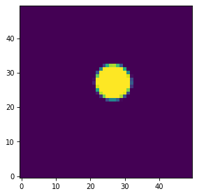
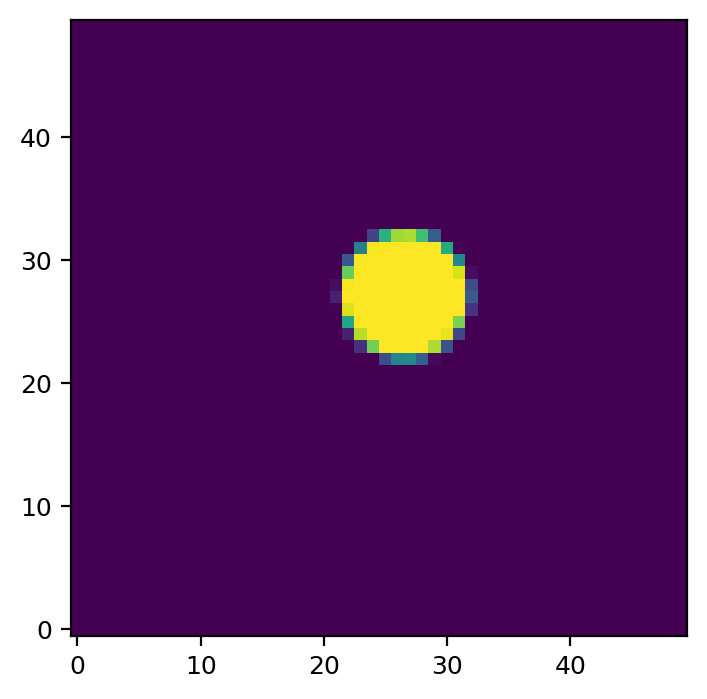
Defining a region mask within an image
RegionMask objects also have a number of
methods to make it easy to use the masks with data. The
to_image() method can be used to obtain an
image of the mask in a 2D array of the given shape. This places the
mask in the correct place in the image and deals properly with boundary
effects. For this example, let’s place the mask in an image with shape
(50, 50):
import matplotlib.pyplot as plt
from regions.core import PixCoord
from regions.shapes.circle import CirclePixelRegion

center = PixCoord(26.6, 27.2)
reg = CirclePixelRegion(center, 5.2)

mask = reg.to_mask(mode='exact')
plt.figure(figsize=(4, 4))
shape = (50, 50)
plt.imshow(mask.to_image(shape), cmap=plt.cm.viridis,
           interpolation='nearest', origin='lower')
(Source code, png, hires.png, pdf, svg)
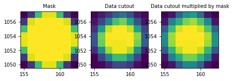
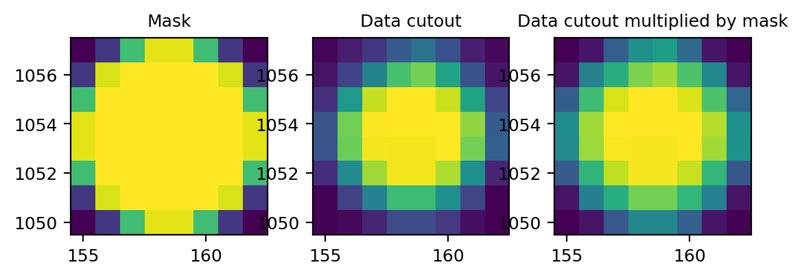
Making image cutouts and multiplying the region mask
The cutout() method can be used to create a
cutout from the input data over the mask bounding box, and the
multiply() method can be used to multiply
the aperture mask with the input data to create a mask-weighted data
cutout. All of these methods properly handle the cases of partial or
no overlap of the aperture mask with the data.
These masks can be used, for example, as the building blocks for photometry, which we demonstrate with a simple example. We start off by getting an example image:
>>> from astropy.io import fits
>>> from astropy.utils.data import get_pkg_data_filename
>>> filename = get_pkg_data_filename('photometry/M6707HH.fits')
>>> hdulist = fits.open(filename)
>>> hdu = hdulist[0]
We then define a circular aperture region:
>>> from regions.core import PixCoord
>>> from regions.shapes.circle import CirclePixelRegion
>>> center = PixCoord(158.5, 1053.5)
>>> aperture = CirclePixelRegion(center, 4.)
We then convert the aperture to a mask and extract a cutout from the data, as well as a cutout with the data multiplied by the mask:
>>> mask = aperture.to_mask(mode='exact')
>>> data = mask.cutout(hdu.data)
>>> weighted_data = mask.multiply(hdu.data)
Note that weighted_data will have zeros where the mask is zero; it
therefore should not be used to compute statistics (see Masked
Statistics below). To get the mask-weighted pixel
values as a 1D array, excluding the pixels where the mask is zero,
use the get_values() method:
>>> weighted_data_1d = mask.get_values(hdu.data)
>>> hdulist.close()
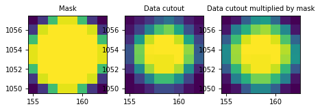
We can take a look at the results to make sure the source overlaps with the aperture:
>>> import matplotlib.pyplot as plt
>>> plt.subplot(1, 3, 1)
>>> plt.title("Mask", size=9)
>>> plt.imshow(mask.data, cmap=plt.cm.viridis,
...            interpolation='nearest', origin='lower',
...            extent=mask.bbox.extent)
>>> plt.subplot(1, 3, 2)
>>> plt.title("Data cutout", size=9)
>>> plt.imshow(data, cmap=plt.cm.viridis,
...            interpolation='nearest', origin='lower',
...            extent=mask.bbox.extent)
>>> plt.subplot(1, 3, 3)
>>> plt.title("Data cutout multiplied by mask", size=9)
>>> plt.imshow(weighted_data, cmap=plt.cm.viridis,
...            interpolation='nearest', origin='lower',
...            extent=mask.bbox.extent)
(Source code, png, hires.png, pdf, svg)
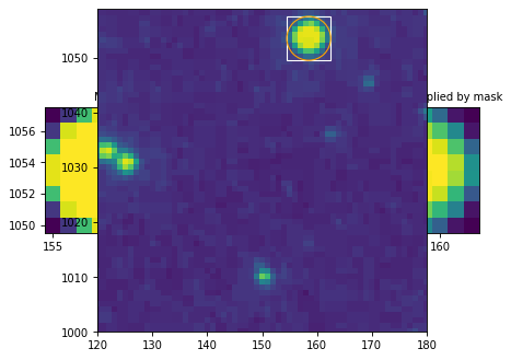
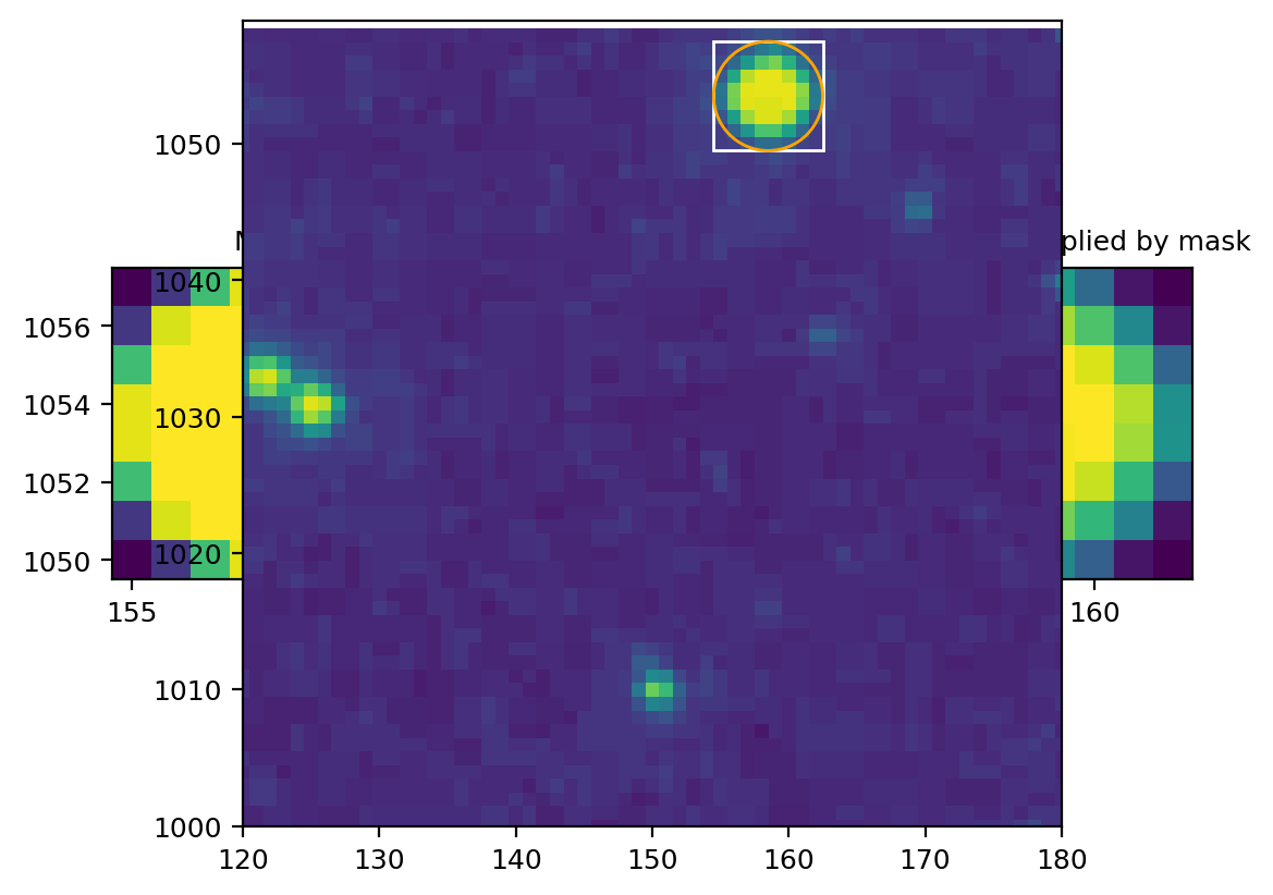
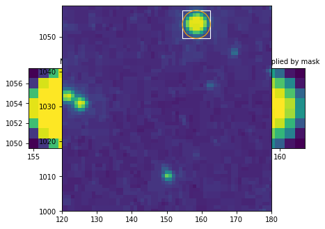
We can also use the RegionMask bbox attribute to look
at the extent of the mask in the image:
from astropy.io import fits
from astropy.utils.data import get_pkg_data_filename
import matplotlib.pyplot as plt
from regions.core import PixCoord
from regions.shapes.circle import CirclePixelRegion

filename = get_pkg_data_filename('photometry/M6707HH.fits')
hdulist = fits.open(filename)
hdu = hdulist[0]
center = PixCoord(158.5, 1053.5)
aperture = CirclePixelRegion(center, 4.)
mask = aperture.to_mask(mode='exact')

ax = plt.subplot(1, 1, 1)
ax.imshow(hdu.data, cmap=plt.cm.viridis,
          interpolation='nearest', origin='lower')
ax.add_artist(mask.bbox.as_artist(facecolor='none', edgecolor='white'))
ax.add_artist(aperture.as_artist(facecolor='none', edgecolor='orange'))
ax.set_xlim(120, 180)
ax.set_ylim(1000, 1059)
hdulist.close()
(Source code, png, hires.png, pdf, svg)
Masked Statistics
Finally, we can use the mask and data values to compute weighted statistics:
>>> import numpy as np
>>> np.average(data, weights=mask)
9364.012674888021
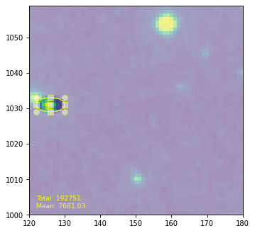
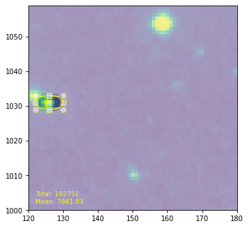
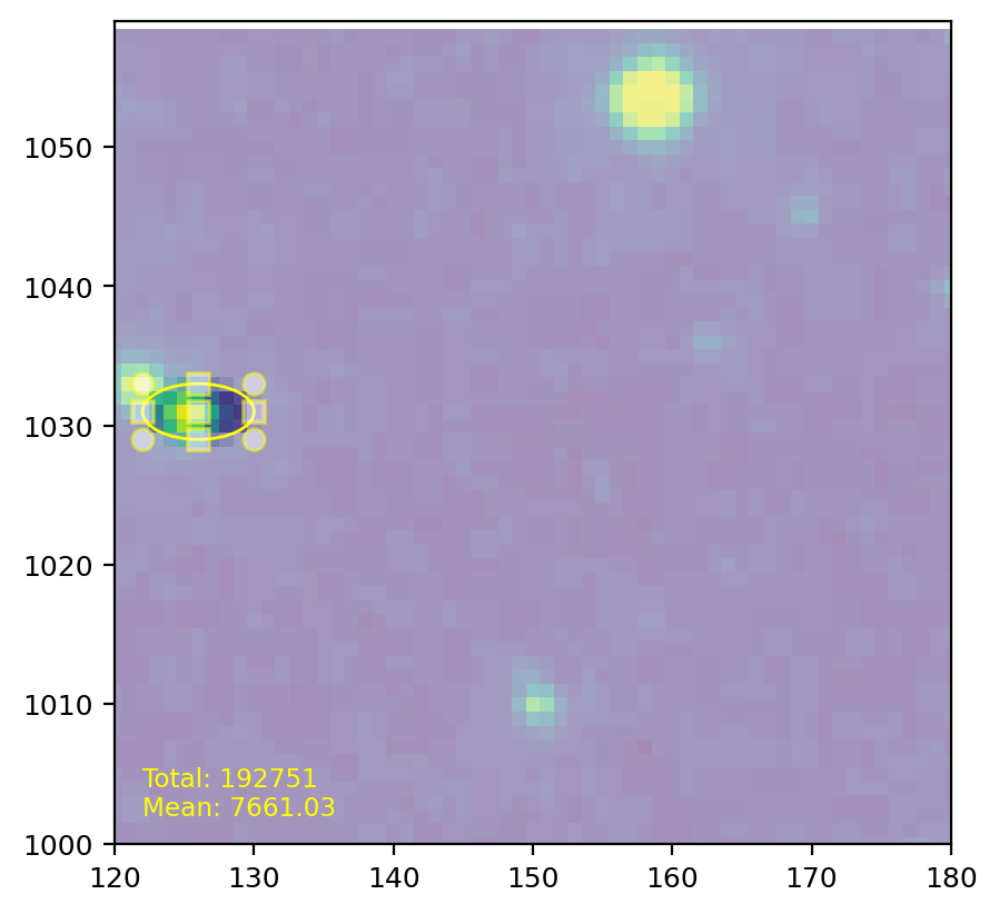
Interactive Mask Control
In the last example we will show how to use a
Matplotlib selector widget with a custom
callback function for creating a mask and updating it interactively through
the selector.
We first create an EllipsePixelRegion and add an as_mpl_selector
property linked to the Matplotlib axes. This can be moved around to
position it on different sources, and resized just like its Rectangle
counterpart, using the handles of the bounding box.
The user-defined callback function here generates a mask from this region and overlays it on the image as an alpha filter (keeping the areas outside shaded). We will use this mask as an aperture as well to calculate integrated and averaged flux, which is updated live in the text field of the plot as well.
from astropy import units as u
from regions import PixCoord, EllipsePixelRegion

hdulist = fits.open(filename)
hdu = hdulist[0]

plt.clf()
ax = plt.subplot(1, 1, 1)
im = ax.imshow(hdu.data, cmap=plt.cm.viridis, interpolation='nearest', origin='lower')
text = ax.text(122, 1002, '', size='small', color='yellow')
ax.set_xlim(120, 180)
ax.set_ylim(1000, 1059)

def update_sel(region):
    mask = region.to_mask(mode='subpixels', subpixels=10)
    im.set_alpha((mask.to_image(hdu.data.shape) + 1) / 2)
    total = mask.multiply(hdu.data).sum()
    mean = np.average(hdu.data, weights=mask.to_image(hdu.data.shape))
    text.set_text(f'Total: {total:g}\nMean: {mean:g}')

ellipse = EllipsePixelRegion(center=PixCoord(x=126, y=1031), width=8, height=4,
                             angle=-0*u.deg, visual={'color': 'yellow'})
selector = ellipse.as_mpl_selector(ax, callback=update_sel)

hdulist.close()
(Source code, png, hires.png, pdf, svg)